Subroutines

Introduction

Syntax

QCL provides 4 kinds of subroutines: classical functions, pseudo-classical operators (qufunct), general unitary operators (operator) and procedures (procedure). The basic syntax for all subroutine declarations is

$$\begin{eqnarray*} \,\mbox{\it def}\, &\leftarrow &(\,\mbox{\it type}\,\vert\,\m... ...}\, \right\} \left\{ \,\mbox{\it stmt}\, \right\}{\tt\verb*=}=} \end{eqnarray*}$$

Hierarchy of Subroutines

Since QCL allows for the inverse call of operators and can perform scratch-space management for quantum functions, the allowed side effects on the classical program state as well as on the quantum machine state have to be strictly specified.

Table 2.11: hierarchy of QCL Subroutines and allowed side-effects

routine type	program state	machine state
procedure	all	all
operator	none	unitary
qufunct	none	pseudo-classic
functions	none	none

The 4 QCL routine types form a call hierarchy, which means that a routine may invoke only subroutines of the same or a lower level (see table 2.11).

The mathematical semantic of QCL operators and functions requires that every call is reproducable. This means, that not only the program state must not be changed by these routines, but also that their execution may in no way depend on the global program state which includes global variables, options and the state of the internal random nuber generator.^2.6

External Routines

While QCL incorporates a classical programming language, to provides all the necessary means to change the program state, there is no hardwired set of elementary operators to manipulate the quantum machine state, since this would require assumptions about the architecture of the simulated quantum computer.

An elementary operator or qufunct can be incorporated by declaring it as extern.

$$\begin{eqnarray*} \,\mbox{\it def}\, &\leftarrow &\,\mbox{\tt extern}\,\,\mbox{... ...\,\mbox{\it identifier}\,\,\mbox{\it arg-list}\,\,\mbox{\tt ;}\, \end{eqnarray*}$$

External operators have no body since they are not executed within QCL, but merely serve as a hook for a binary function which implements the desired operation directly by using the numeric QC-library [17] and is linked to the interpreter.

The interpreter qcl includes binary versions of several common operators, including an implementation of the Fanout operator (see section 2.5.6.2) which is used by QCL scratch space management, and patterns of general unitary matrices to allow the implementation of new elementary operators.

To conveniently define a custom set of elementary operators, the external declarations can be included into the default include file default.qcl. Note that a definition of a Fanout has to be provided if local scratch variables are to be used.

For a complete list of available external operators, please refer to section 3.1.

Functions

Functions are the most restrictive routine type and don't allow any interactions with the global state.

User defined functions may be of any classic type, namely int, real, complex or string, and may take an arbitrary number of classical parameters. The value of the function is passed to the invoking routine by the return statement.

int digits(int n) {           // calculate the number of
  return 1+floor(log(n,2));   // binary digits of n
}

Lokal variables can be defined at the top of the function body.

int fibonachi(int n) {       // calculate the n-th
      int a=0;               // fibonachi number
      int b=1;               // by iteration
      int i;
      for i = 1 to n {
              b = a+b;
              a = b-a;
      }
      return a;
}

Functions can call other functions within their body. Recursive calls are also allowed.

int fac(int n) {              // calculate n!
  if n<2 {                    // by recursion
    return 1;
  } else {
    return n*fac(n-1);
  }
}

Other than most internal functions, no implicit typecasting is performed, so the function arguments have to exactly match the specified parameter type.

Procedures

Procedures are the most general routine type and used to implement the classical control structures of quantum algorithms which generally involve evaluation loops, the choise of applied operators, the interpretation of measurements and classical probabilistic elements.

With the exception of routine declarations, procedures allow the same operations as are available in global scope (e.g. at the shell prompt) allowing arbitrary changes to both the program and the machine state. Operations exclusive to procedures are

• Access to global variables
• (Pseudo) Random numbers by using the pseudo-function random (see section 2.2.3.7)
• Non-unitary operations on the machine state by using the reset and measure commands (see section 2.4.2.2)
• User input by using the input command (see section 2.4.1.3)

Procedures can take any number of classical or quantum arguments and may call all types of subroutines.

procedure prepare(qureg q) {
  const l = #q/2;        // use one half of the register
  int i;                 // for the offset
  reset;                 // initialize machine state
  Mix(q[l:#q-1]);        // generate periodic distribution
  for i = 0 to l-1 {     // randomize the offset
    if 0.5<random() {
      Not(q[i]);
    }
  }
}

The procedure prepare generates a periodic test state with random offset, as we have used in the DFT example in section 2.1.2.

qcl> qureg q[4];
qcl> prepare(q);
[4/4] 0.5 |0010> + 0.5 |1010> + 0.5 |0110> + 0.5 |1110>
qcl> prepare(q);
[4/4] 0.5 |0000> + 0.5 |1000> + 0.5 |0100> + 0.5 |1100>
qcl> prepare(q);
[4/4] 0.5 |0011> + 0.5 |1011> + 0.5 |0111> + 0.5 |1111>

Procedures may declare local variables of classical and quantum types. When local quantum registers are used, it is up to the programmer to properly empty them again, which can either be acheived by uncomputing or by a reset command. Table 2.12 shows a simple game where a local quantum register is used to generate ``real'' random numbers.

Table 2.12: roulette.qcl quantum roulette

General Operators

The routine type operator is used for general unitary operators. Conforming to the mathematical notion of an operator, a call with the same parameters has to result in exactly the same transformation, so no global variable references, random elements or dependencies on input are allowed.

Since the type operator is restricted to reversible transformations of the machine state, reset and measure commands are also forbidden.

Operator Arguments

Operators work on one or more quantum registers (register operator, see section 1.3.2.2), so depending on the mapping of the registers, a call of an $m$ qubit operator with a total quantum heap of $n$ qubits can result in $\frac{n!}{(n-m)!}$ different unitary transformations.

In QCL, this polymorphism is even further extended by the fact, that quantum registers can be of different sizes, so for every quantum parameter $\mathbf{s}$, the register size ${\tt\char93 }\mathbf{s}=\vert\mathbf{s}\vert$ is an implicit extra parameter of type int. An addition to that, operators can take an arbitrary number of explicit classical arguments.

If more than one argument register is given, their qubits may not overlap.

qcl> qureg q[4];
qcl> qureg p=q[2:3];
qcl> CNot(q[1\2],p);
! runtime error: quantum arguments overlapping

Inverse Operators

As allready mentioned in section 2.4.1.2, operator calls can be inverted by the adjungation prefix `!'. The adjoint operator to a composition of unitary operators is^2.7

$$\left(\,\prod_{i=1}^{n}U_i\right)^\dagger = \prod_{i=n}^1U^\dagger _i$$ (2.10)

Since the sequence of applied suboperators is specified using a procedural classical language which cannot be executed in reverse, the inversion the composition, is is achieved by the delayed execution of operator calls.

When the adjungation flag is set, the operator body is executed and all calls of suboperators are pushed on a stack which is then processed in reverse order with inverted adjungation flags.

Local Registers

As opposed to pseudo-classic operators, it is in general impossible to uncompute an unitary operator in order to free a local register again without also destroying the intended result of the computation. This is a fundamental limitation of QC known as the non cloning theorem which results from the fact that a cloning operation i.e. a transformation with meets the condition

$$U: {\vert\psi \rangle}{\vert \rangle}\to{\vert\psi \rangle}{\vert\psi \rangle}$$ (2.11)

for an arbitrary^2.8 ${\vert\psi \rangle}$ cannot be unitary if ${\vert\psi \rangle}$ is a composed state because

$$U\,( a{\vert,0 \rangle}+b{\vert 1,0 \rangle})= a^2{\vert,0 \rangle}+ab\,{\vert,1 \rangle}+ba\,{\vert 1,0 \rangle})+b^2{\vert 1,1 \rangle}$$ (2.12)

$$\neq a\,U\,{\vert,0 \rangle}+b\,U\,{\vert 1,0 \rangle}= a{\vert,0 \rangle}+b{\vert 1,1 \rangle}$$ (2.13)

$U$ can only be unitary if ${\vert\psi \rangle}$ is in a pure state, i.e. ${\vert\psi \rangle}={\vert i \rangle}$, in which case $U=\mathit{FANOUT}$.

Due to the lack of a unitary copy operation for quantum states, Bennet-style scratch space management is impossible for general operators since it is based on cloning the result register.

Despite this limitation, it is possible in QCL to allocate temporary quantum registers but it is up to the programmer to properly uncompute them again. If the option -check is set, proper cleanup is verified by the simulator.

qcl> set check 1 
qcl> operator foo(qureg q) { qureg p[1]; CNot(p,q); }
qcl> qureg q[1];
qcl> Mix(q);
[1/4] 0.707107 |0000> + 0.707107 |0001>
qcl> foo(q);
! in operator foo: memory error: quantum heap is corrupted
[1/4] 0.707107 |0000> + 0.707107 |0011>

Local registers are useful if an operator contains some intermediary pseudo-classic operations which require scratch space. See the implementation of modular addition (addn) in section 3.2.2.1 (page ) for an example.

Pseudo-classic Operators

The routine type qufunct is used for pseudo-classic operators and quantum functions, so all transformations have to be of the form

$${\vert\Psi \rangle}=\sum_i c_i {\vert i \rangle} \to \sum_{i,j} c_i \delta_{j\pi_i} {\vert j \rangle}={\vert\Psi' \rangle}$$ (2.14)

with some permutation $\pi$. All $n$ qubit pseudo-classic operators $F$ therefore have the common eigenstate

$${\vert\Psi \rangle}=2^{-\frac{1}{2}n} \sum_{i=0}^{2^n-1}{\v... ...ngle} \Rightarrow F\,{\vert\Psi \rangle}={\vert\Psi \rangle}$$ (2.15)

Bijective Functions

The most straightforward application for pseudo-classic operators is the direct implementation of bijective functions (see section 1.3.3.1)

qufunct inc(qureg x) {
  int i;
  for i = #x-1 to 1 {
    CNot(x[i],x[0:i-1]);
  }
  Not(x[0]);
}

The operator inc shifts the base-vectors of it's argument. In analogy to boson states, where the increment of the eigenstate corresponds to the generation of a particle, inc is a creation operator.^2.9

qcl> qureg q[4];
qcl> inc(q);
[4/4] 1 |0001>
qcl> inc(q);
[4/4] 1 |0010>
qcl> inc(q);
[4/4] 1 |0011>
qcl> inc(q);
[4/4] 1 |0100>

Conditional Operators

When it comes to more complicated arithmetic operations, it is often required to apply a transformation to a register $\mathbf{a}$ in dependence on the content of another register $\mathbf{e}$.

If all qubits of $\mathbf{e}$ are required to be set, for the transformation to take place, the operator is a conditional operator with the invariant (quconst) enable register $\mathbf{e}$ (see section 1.3.5).

A simple example for a conditional operator is the Toffoli gate $T:{\vert x,y,z \rangle}\to{\vert x\oplus (y\wedge z),y,z \rangle}$ or it's generalisation, the controlled not gate. A conditional version of the above increment operator is also easy to implement:

qufunct cinc(qureg x,quconst e) {
  int i;
  for i = #x-1 to 1 step -1 {
    CNot(x[i],x[0:i-1] & e);
  }
  CNot(x[0],e);
}

Now, only base-vectors of the form ${\vert i \rangle}{\vert 11\ldots \rangle}_\mathbf{s}$ are incremented:

qcl> qureg q[4]; qureg e[2]; Mix(e);
[6/6] 0.5 |000000> + 0.5 |100000> + 0.5 |010000> + 0.5 |110000>
qcl> cinc(q,e);
[6/6] 0.5 |000000> + 0.5 |100000> + 0.5 |010000> + 0.5 |110001>
qcl> cinc(q,e);
[6/6] 0.5 |000000> + 0.5 |100000> + 0.5 |010000> + 0.5 |110010>
qcl> cinc(q,e);
[6/6] 0.5 |000000> + 0.5 |100000> + 0.5 |010000> + 0.5 |110011>

Quantum Functions

As defined in section 1.3.3.2, a quantum function $F$ is a pseudo-classic operator with the characteristic

$$F:{\vert x \rangle}_\mathbf{x}{\vert \rangle}_\mathbf{y}\to... ...e}_\mathbf{y} \quad{\rm with}\quad f:{\bf B}^n \to {\bf B}^m$$ (2.16)

If we require the argument register $\mathbf{x}$ to be invariant to $F$ by declaring $\mathbf{x}$ as quconst, this leaves us with $2^{(2^n-1)m}$ possible pseudo-classic implementations of $F$ for any given $f$. To reflect the fact that $F\,{\vert x,y\neq 0 \rangle}$ is undefined, the target register has to be of type quvoid. (see section 2.3.2.3).

Since, according to the above definition, quantum functions are merely ordinary pseudo-classic operators, whose specification is restricted to certain types of input states, they also use the same QCL routine type qufunct.

The following example calculates the parity of $\mathbf{x}$ and stores it to $\mathbf{y}$:

qufunct parity(quconst x,quvoid y) {
  int i;
  for i = 0 to #x-1 {
    CNot(y,x[i]);
  }
}

qcl> qureg x[2]; qureg y[1]; Mix(x);
[3/3] 0.5 |000> + 0.5 |010> + 0.5 |001> + 0.5 |011>
qcl> parity(x,y);
[3/3] 0.5 |000> + 0.5 |110> + 0.5 |101> + 0.5 |011>

Scratch parameters

We can extend the notion of quantum functions, by also allowing an explicit scratch register $\mathbf{s}$ (see section 2.3.2.4) as an optional parameter to $F$, so we end up with an operator $F(\mathbf{x},\mathbf{y},\mathbf{s})$ with the characteristic

$$F:{\vert x \rangle}_\mathbf{x}{\vert \rangle}_\mathbf{y}{\v... ...bf{x}{\vert f(x) \rangle}_\mathbf{y}{\vert \rangle}_\mathbf{s}$$ (2.17)

Using the parity and the cinc operator form the above examples, we can implement an ``add parity'' function $f(x)=x+\mathrm{parity}(x)$ by providing a scratch qubit:

qufunct addparity(quconst x,quvoid y,quscratch s) {
  parity(x,s);      // write parity to scratch
  x -> y;           // Fanout x to y
  cinc(y,s);        // increment y if parity is odd
  parity(x,s);      // clear scratch
}

qcl2> qureg x[2]; qureg y[2]; qureg s[1]; Mix(x);
[5/8] 0.5 |00000> + 0.5 |00010> + 0.5 |00001> + 0.5 |00011>
qcl2> addparity(x,y,s);
[5/8] 0.5 |00000> + 0.5 |01110> + 0.5 |01001> + 0.5 |01111>

Instead of providing a explicit scratch parameter, we can, of course, also use a local register of type qureg, which is functionally equivalent:

qufunct addparity2(quconst x,quvoid y) {
  qureg s[1];
  parity(x,s);
  x -> y;
  cinc(y,s);
  parity(x,s);
}

qcl2> qureg x[2]; qureg y[2]; Mix(x);
[4/8] 0.5 |00000> + 0.5 |00010> + 0.5 |00001> + 0.5 |00011>
qcl2> addparity2(x,y);
[4/8] 0.5 |00000> + 0.5 |01110> + 0.5 |01001> + 0.5 |01111>

Explicit scratch parameters are useful to save memory, if a quantum function $F$ is to be used by another operator $U$, which still has empty scratch registers at the moment, the suboperator is called, which would e.g. be the case if $U$ is of the form

$$U(\mathbf{x},\mathbf{y},\mathbf{s},\ldots)= \left(\prod_{i... ...f{x},\mathbf{y},\mathbf{s})\,U_1(\mathbf{x},\mathbf{y},\ldots)$$ (2.18)

Since both, explicit scratch parameters of type quscratch and local registers of type qureg, have to be uncomputed manually, they are especially useful for quantum functions $U:{\vert x,0,0 \rangle}\to {\vert x,f(s(x),x),0 \rangle}$ of the form

$$U(\mathbf{x},\mathbf{y},\mathbf{s})=S(\mathbf{x},\mathbf{s}... ...hbf{x},\mathbf{s},\mathbf{y})S^\dagger (\mathbf{x},\mathbf{s})$$ (2.19)

if $S$ is invariant to $\mathbf{x}$ and $F$ is invariant to $\mathbf{x}$ and $\mathbf{s}$, because the uncomputation of $\mathbf{s}$ doesn't require an additional register to temporarily save $\mathbf{y}$ (see section 1.3.4.2) as would be the case, if a managed local scratch register of type quscratch would be used instead (see below).

The Fanout Operator

The restriction to base-vector permutations implies that the computational path of a pure state is also a sequence of pure states, so in the case of superpositions each base-vector can be treated separately.

As shown in section 2.5.4, a arbitrary pure state ${\vert\psi \rangle}={\vert i \rangle}$ can be copied onto an empty register by a unitary $\mathit{FANOUT}$ operation:

$$\mathit{FANOUT}: {\vert\psi \rangle}{\vert \rangle}={\vert ... ...}\to{\vert i,i \rangle}={\vert\psi \rangle}{\vert\psi \rangle}$$ (2.20)

For non-empty target registers, $\mathit{FANOUT}\,{\vert i,j\neq 0 \rangle}$ is undefined, so for two $n$ qubit registers there are $(2^{2n}-2^n)!$ possible pseudo-classic implementations of a fanout gate.^2.10

Table 2.13 shows a realisation using controlled-not gates which is mathematically equivalent to the default implementation of the external operator Fanout.

Table 2.13: fanout.qcl Custom implementation of Fanout

Scratch Space Management

The quantum type quscratch declares a local register as managed scratch space. Managed scratch space (or junk) registers are temporary registers which are empty when allocated and automatically get uncomputed after the body of the qufunct has been applied.

So, in contrast to local qureg registers or quscratch parameters, a local quscratch register $\mathbf{j}$ has not to be emptied within the the qufunct definition but can be left dirty. So, in order to compute some $f(x)$, it is sufficient, the the body of the quantum function merely implements some operator $F:{\vert x,0,0 \rangle}\to{\vert x,f(x),j(x) \rangle}$ with an arbitrary junk string $j(x)$ in the scratch register.

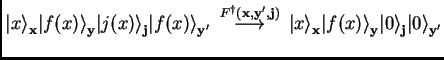
When a quantum function with the local junk register $\mathbf{j}$ and the body $F(\mathbf{x},\mathbf{y},\mathbf{j})$ is called, an additional scratch register $\mathbf{y'}$ of the same size as $\mathbf{y}$ is allocated and instead of the 3 register operator $F$, the 4 register operator $F'$ is applied, which is defined as

$$F'(\mathbf{x},\mathbf{y},\mathbf{j},\mathbf{y'})= F^\dagge... ...mathbf{y'},\mathbf{y})\, F(\mathbf{x},\mathbf{y'},\mathbf{j})$$ (2.21)

$F'$ initially calls $F$, but instead of $\mathbf{y}$, a temporary target register $\mathbf{y'}$ is used. The desired result $f(x)$ is then copied onto the original target register $\mathbf{y}$, while the undesired junk result $j(x)$ is left in the junk register. By undoing the initial computation by applying the adjoint operator $F^\dagger$, both, the junk register $\mathbf{j}$ and the scratch register $\mathbf{y'}$, get uncomputed again, so the whole procedure is:

$${\vert x \rangle}_\mathbf{x}{\vert \rangle}_\mathbf{y}{\vert \rangle... ...hbf{y'} \,\stackrel{\mathit{FANOUT}(\mathbf{y'},\mathbf{y})}{\longrightarrow}\,$$ (2.22)

$${\vert x \rangle}_\mathbf{x}{\vert f(x) \rangle}_\mathbf{y}{\vert j(... ...t f(x) \rangle}_\mathbf{y}{\vert \rangle}_\mathbf{j}{\vert \rangle}_\mathbf{y'}$$

By using the conditional increment operator from page we can construct a quantum function bitcmp which implements a ``bit comparison'' function $f(x_1,x_2)$ which returns 1 if the bitstrings $x_1$ and $x_2$ contain the same number of set bits, and zero otherwise.

qufunct bitcmp(quconst x1,quconst x2,quvoid y) {
  const n=ceil(log(max(#x1,#x2)+1,2));
  int i;
  quscratch j[n];        // allocate a managed scratch register
  for i=0 to #x1-1 {     // j = number of bits in x1
    cinc(j,x1[i]);       // increment j if bit i of x1 is set
  }
  Not(j);                // j = 2^n-j-1 = -1-j mod 2^n
  for i=0 to #x2-1 {     // j = j+number of bits in x2
    cinc(j,x2[i]);       // increment j if bit i of x1 is set
  }
  CNot(y,j);             // set y=1 if j==2^n-1
}

qcl> qureg x1[2]; qureg x2[2]; qureg y[1];
qcl> Mix(x1[1]); Mix(x2[0]); Not(x2[1]);
[5/8] 0.5 |00001000> + 0.5 |00001100> + 0.5 |00001010> + 0.5 |00001110>
qcl> bitcmp(x1,x2,y);
[5/8] 0.5 |00001000> + 0.5 |00001100> + 0.5 |00011010> + 0.5 |00001110>

By using the option -log we can trace the call of each elementary operator:

qcl> set log 1
qcl> bitcmp(x1,x2,y);
@ CNot(qureg q=|0.......>,quconst c=|.0.....1>)
@ CNot(qureg q=|.0......>,quconst c=|.......0>)
@ CNot(qureg q=|0.......>,quconst c=|.0....1.>)
@ CNot(qureg q=|.0......>,quconst c=|......0.>)
@ Not(qureg q=|10......>)
@ CNot(qureg q=|0.......>,quconst c=|.0...1..>)
@ CNot(qureg q=|.0......>,quconst c=|.....0..>)
@ CNot(qureg q=|0.......>,quconst c=|.0..1...>)
@ CNot(qureg q=|.0......>,quconst c=|....0...>)
@ CNot(qureg q=|..0.....>,quconst c=|10......>)
@ Fanout(quconst a=|..0.....>,quvoid b=|...0....>)
@ !CNot(qureg q=|..0.....>,quconst c=|10......>)
@ !CNot(qureg q=|.0......>,quconst c=|....0...>)
@ !CNot(qureg q=|0.......>,quconst c=|.0..1...>)
@ !CNot(qureg q=|.0......>,quconst c=|.....0..>)
@ !CNot(qureg q=|0.......>,quconst c=|.0...1..>)
@ !Not(qureg q=|10......>)
@ !CNot(qureg q=|.0......>,quconst c=|......0.>)
@ !CNot(qureg q=|0.......>,quconst c=|.0....1.>)
@ !CNot(qureg q=|.0......>,quconst c=|.......0>)
@ !CNot(qureg q=|0.......>,quconst c=|.0.....1>)

The first 10 operations belong to the body operator $F$; after the $\mathit{FANOUT}$, they are repeated in reverse order with inverted adjungation flags ($F^\dagger$).

By additionally using the option -log-state, we can also trace the evolution of the machine state.

qcl> bitcmp(x1,x2,y);
@ CNot(qureg q=|0.......>,quconst c=|.0.....1>)
% 0.5 |00001000> + 0.5 |00001100> + 0.5 |00001010> + 0.5 |00001110>
.....
% 0.5 |00001000> + 0.5 |01001100> + 0.5 |11101010> + 0.5 |00001110>
@ Fanout(quconst a=|..0.....>,quvoid b=|...0....>)
% 0.5 |00001000> + 0.5 |01001100> + 0.5 |11111010> + 0.5 |00001110>
.....
@ !CNot(qureg q=|0.......>,quconst c=|.0.....1>)
% 0.5 |00001000> + 0.5 |00001100> + 0.5 |00011010> + 0.5 |00001110>

Footnotes

... generator.^2.6

These restrictions can be partially overridden for debugging purposes by using the shell command

... is^2.7

To avoid ambiguities with non-commutative matrix products, we use the convention $\prod_{i=1}^n f_i=f_nf_{n-1}\ldots f_1$

... arbitrary^2.8

For any particular ${\vert\psi \rangle}$ an infinite number of unitary ``cloning'' operators trivially exists, as e.g. $U_\psi=\sum_{i,j,k} {\vert i,j\oplus k \rangle}{\langle k\vert\psi \rangle}{\langle i,j\vert}$

... operator.^2.9

In fact, this is not quite correct, since other than bosons, an $n$ qubit register is limited to $2^n$ states, so $\mathtt{inc}\,{\vert 2^n-1 \rangle}={\vert \rangle}$ whereas $a^\dagger \,{\vert 2^n-1 \rangle}={\vert 2^n \rangle}$

... gate.^2.10

In fact, the definition of fanout used by QCL is somewhat more restrictive, since it requires the first argument to be invariant (quconst). This can be overridden be redeclaring the argument as qureg if necessary (see section 2.3.2.5)