Wave Mechanics

Classical States

In classical physics, the momentary state of a particle is given by it's location $\vec{r}$ and it's velocity $\vec{v}$.

When we talk about the temporal behavior of dynamic systems, however, this notion of ``state'' is somewhat cumbersome to deal with, since by definition, the momentary state of the system changes constantly. This is especially true when it comes to periodic movement, so it is often more adequate to talk about the current orbit of a satellite (which remains constant until it is actively altered by outside intervention) than to give the actual coordinates (which permanently change).

So in a more abstract definition, the states of an isolated classical system are the positions $\vec{r}_1, \vec{r}_2,\ldots$ of all included particles as a function of time $t$.^1.2

State Changes

The above definition implies that the state of a system can only change when an interaction with another system occurs.

Typically, the duration of the interaction (e.g. the collision of 2 billiard-balls) is very small compared to the duration of the isolated states, so for practical purposes the interaction can often be assumed as instantaneous.

Conservation Laws

Isolated systems preserve their total energy $E$ and momentum^1.3 $\vec{p}$, which are given as^1.4

$$E=V(\vec{r}_1, \vec{r}_2,\ldots)+\sum_i m_i v^2_i \quad\mathrm{and}\quad \vec{p}=\sum_i m_i \vec{v}_i$$ (1.4)

Thus, states can be characterized by these quantities and often the total energy of a state is much more interesting than the state itself.

Movement Laws

Legal physical states must obey a movement law which characterizes the dynamics of a system. For classic one-particle systems, the dynamic equation is known as Newton's Second Law

$$m \frac{\partial^2 \vec{r}}{\partial t^2}=\vec{F}(\vec{r},t)$$ (1.5)

For conservative fields such as non relativistic gravitational and static electric fields, the force $\vec{F}$ is the negative gradient of a scalar potential $V(\vec{r})$, thus the equation above can be written as

$$m \frac{\partial^2 \vec{r}}{\partial t^2}=-\mathrm{grad} V(\vec{r})$$ (1.6)

Any momentary state of the system can be used as an initial value for the above equation to determine its temporal behavior.

The Wave Function

In quantum physics, the state of a one-particle system is characterized by a complex distribution function $\psi(\vec{r},t)$ with the normalization

$$\int\vert\psi(\vec{r},t)\vert^2 d^3\vec{r}=1$$ (1.7)

Two states differing by a constant phase factor $\mathrm{e}^{\mathrm{i}\phi}$ are considered equivalent.

Particle Location

The classical notion of particle location is replaced by a spatial probability distribution $\rho={\psi}^*\psi$, which can be characterized by its expectation value ${\langle \vec{r} \rangle}$ and its uncertainty $\Delta r$, which are defined as

$${\langle \vec{r} \rangle}=\int{\psi}^*(\vec{r},t)\vec{r}\ps... ...lta r=\sqrt{{\langle r^2 \rangle}-{\langle \vec{r} \rangle}^2}$$ (1.8)

Time Dependency

When a classical system involves moving particles, the location of the particles is time dependent. This is not necessarily the case with quantum systems and the describing probability distribution $\rho$: If the quantum state $\psi$ is of the form $\psi(\vec{r},t)=\psi(\vec{r})\phi(t)$ with $\vert\phi(t)\vert=1$, then $\rho={\psi}^*(\vec{r})\psi(\vec{r})$ is time independent.

Figure 1.1 shows a particle that is trapped between two reflecting ``mirrors''.<sup>1.5</sup>A classical particle will move periodically from on end to another at a constant speed, it's location can be described by a periodic triangle-function of the time. An undisturbed quantum particle in a similar trap, however, doesn't have a defined location; the probability to ``meet'' (i.e. measure) the particle at a certain location remains constant over time^1.6but changes throughout space, or in more physical terms, the particle forms a standing wave just as a vibrating piano-string between 2 fixed ends.

Figure 1.1: A ball trapped between two mirrors as classical and as quantum particle

A constant probability distribution is typical for bound states of defined energy, i.e. for particles trapped in a constant potential well, e.g. an electron in the electric field of a proton.

Expectation Values

It has been shown above how the classical concept of a well defined particle location has been replaced by the quantum concept of a statistical expectation value. This correspondence, however, is not just restricted to space. In fact, all classical physical quantities of a system can be described as the expectation value of an appropriate operator (see table 1.1 for some examples).

Table 1.1: Some observables and their corresponding operators

Observable	classical value	Operator
Location	$\vec{r}$	$\vec{R}=\vec{r},\;R_i=r_i$
Momentum	$\vec{p}=m \frac{\partial \vec{r}}{\partial t}$	$\vec{P}=-i\hbar \nabla, \; P_i=-i\hbar\frac{\partial }{\partial r_i}$
Angular Momentum	$\vec{L}=\vec{p}\times\vec{r}$	$\vec{\mathcal{L}}=\vec{R}\times\vec{P}, \; {\mathcal{L}}_i=-i{\hbar}\epsilon_{ijk}r_j\frac{\partial }{\partial r_k}$
Energy	$E=\frac{p^2}{2m}+V(\vec{r})$	$H=-\frac{\hbar^2}{2m}\Delta+V$

In analogy to equation 1.2.2.1, the expectation value ${\langle O \rangle}$ and the uncertainty for an observable $\mathcal{O}$ are defined as

$${\langle O \rangle}=\int{\psi}^*(\vec{r},t) O \psi(\vec{r... ... \Delta O=\sqrt{{\langle O^2 \rangle}-{\langle O \rangle}^2}$$ (1.9)

The Schrödinger Equation

The quantum analogy to Newton's Third Law (see equation 1.6) is the Schrödinger Equation

$$H \psi=i\hbar \frac{\partial }{\partial t} \psi$$ (1.10)

which determines the dynamics of a particle system. The Hamilton operator $H$ describes the total energy of the system at a given time and can be very complicated.

The Time-Independent Schrödinger Equation

If we take the simple case of a particle in a static potential field $V$, equation 1.10 can be written as

$$\left(-\frac{\hbar^2}{2m}\nabla^2+V(\vec{r})\right)\psi(\vec{r},t)= i\hbar \frac{\partial }{\partial t} \psi(\vec{r},t)$$ (1.11)

If we split off the time dependent part, using the ansatz $\psi(\vec{r},t)=\psi(\vec{r})\phi(t)$ from 1.2.2.2 and the separation parameter $E$, we get

$$E \phi(t)=i\hbar \frac{\partial }{\partial t} \phi(t) \quad\mathrm{and}\quad H \psi(\vec{r}) = E \psi(\vec{r})$$ (1.12)

The time part is solved by $\phi=\mathrm{e}^{-\mathrm{i}\omega t}$ with $\omega=E/\hbar$. $E$ is the energy of the state, since

$${\langle H \rangle}= \int{\psi}^*(\vec{r})\left(H \psi(\v... ...3\vec{r}= E\int{\psi}^*(\vec{r}) \psi(\vec{r}) d^3\vec{r}=E$$ (1.13)

The remaining eigenvalue problem $E \psi=H \psi$ is also called the time-independent Schrödinger Equation.^1.7

Energy Spectra

Depending on the imposed boundary conditions, the Schrödinger Equation is often only solvable for particular values of $E$, i.e. it has a discrete energy spectrum and the possible eigenvalues $E_n$ (also called energy terms) can be enumerated. The solution for the lowest eigenvalue $E_0$ is called the ground-state $\psi_0$ of the system.

Since for most physical applications, only the value of the energy terms is of importance, it is hardly ever necessary to actually compute the eigenstates.

It has been the discovery of discrete energy states, which gave quantum physics its name, as any state change from eigenstate $\psi_n$ to $\psi_m$ involves the exchange of an energy quantum $\Delta E=E_m-E_n$.

Electron in a Capacitor

As an example, let's consider an electron in a capacitor. To keep things simple, the capacitor should be modeled by an infinitely deep, one-dimensional potential well (see also 1.2.2.2), thus

$$V(\vec{r})=V(x)= \left\{ \begin{array}{cl} 0 & \; \mbox{... ...\; 0<x<l \\ \infty & \;\mbox{otherwise} \end{array}\right.$$ (1.14)

This leads us the the time-independent Schrödinger Equation

$$-\frac{\hbar^2}{2m_e} \psi''(x)=E \psi(x)$$ (1.15)

and the boundary conditions

$$\psi(0)=0 \quad\mathrm{and}\quad \psi(l)=0$$ (1.16)

The ansatz $\psi(x)=N\sin(kx)$ automatically satisfies the first BC and leads to $k=\sqrt{2m_eE}/\hbar$. To satisfy the second BC, we have to introduce the quantization-condition $kl=n\pi$. The normalization constant $N$ has to be chosen such that $\int\vert\psi(x)\vert^2dx=1$, thus the final result is

$$\psi_n(x)=\sqrt{\frac{2}{l}} \sin(k_n x) \quad\mathrm{with}\quad k_n=\frac{\pi}{l}n$$ (1.17)

and the corresponding energies

$$E_n=\frac{\hbar^2k_n^2}{2m_e}=\frac{\pi^2\hbar^2}{2m_el^2}n^2,\quad n=1,2,\ldots\infty$$ (1.18)

The general time dependent solution is

$$\psi(x,t)=\sum_{n=1}^{\infty} c_n \psi_n(x,t) \quad\mathrm{... ...\sum_{n=1}^{\infty} \vert c_n\vert^2=1 \quad\mathrm{and}\quad$$ (1.19)

$$\psi_n(x,t)=\sqrt{\frac{2}{l}} \mathrm{e}^{-\mathrm{i}\ome... ...n x), \quad k_n=\frac{\pi}{l}n, \; \omega_n=\frac{E_n}{\hbar}$$ (1.20)

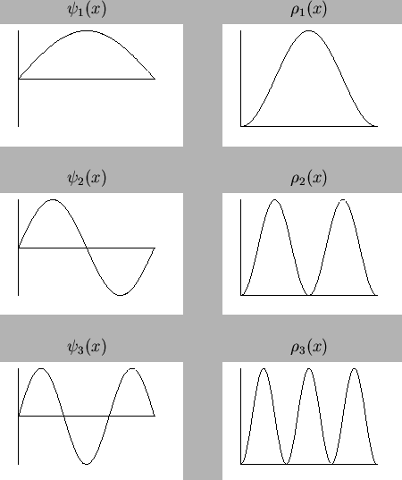
Figure 1.2 shows the first 3 eigenstates $\psi_1, \psi_2$ and $\psi_3$ and their corresponding spatial probability distributions $\rho_n=\vert\psi_n\vert^2$.

Figure 1.2: The first three eigenstates for an electron in a potential well

3-dimensional Trap

The above example can easily be extended to 3 dimensions, using the potential

$$V(\vec{r})=V\left(\begin{array}{c}x y z\end{array}\ri... ...\; 0<z<l \\ \infty & \;\mbox{otherwise} \end{array}\right.$$ (1.21)

This leads to the eigenfunctions

$$\psi_{n_1,n_2,n_3}(\vec{r})= \left(\frac{2}{l}\right)^{\fr... ...}{l}n_1 x) \sin(\frac{\pi}{l}n_2 y) \sin(\frac{\pi}{l}n_3 z)$$ (1.22)

and the energies

$$E_{n_1,n_2,n_3}=E_{n_1+n_2+n_3}= \frac{\pi^2\hbar^2}{2m_el^2}(n_1^2+n_2^2+n_3^2)$$ (1.23)

Since the different states can have the same energy (e.g. $E_{211}=E_{121}=E_{112}$) i.e. the eigenvalues of the Hamilton operator $H$ are degenerated, measuring the energy is not sufficient for determining the actual electron distribution.

Footnotes

....^1.2

Note, that since $\vec{v}=\dot{\vec{r}}=\partial\vec{r}/\partial t$, this also includes the velocities.

... momentum^1.3

There are several other conservation laws for angular momentum, electric charge, baryon count, etc. which are not mentioned here

... as^1.4

The form of the potential energy $V$ actually defines the physical problem and can also depend on particle velocities, time, spins, etc.

... ``mirrors''.^1.5

Mathematically, such ideal ``mirrors'' are described by infinitely deep potential-wells.

... time^1.6

This is only the case with eigenstates; in mixed states, the local probability can oscillate due to the different periods of the involved phase functions $\phi_i(t)$

... Equation.^1.7

Note that this requires the Hamilton operator to be time-independent, which is not necessarily the case