Many problems in classical computer science can be reformulated
as searching a list for a unique element which matches some
predefined condition.
If no additional knowledge about the search-condition ![]() is
available, the best classical algorithm is a brute-force
search i.e. the elements are sequentially tested against
is
available, the best classical algorithm is a brute-force
search i.e. the elements are sequentially tested against ![]() and as soon as an element matches the condition, the
algorithm terminates.
For a list of
and as soon as an element matches the condition, the
algorithm terminates.
For a list of ![]() elements, this requires an average of
elements, this requires an average of
![]() comparisons.
comparisons.
By taking advantage of quantum parallelism and interference,
Grover found a quantum algorithm which can find the matching
element in only ![]() steps. [20]
steps. [20]
The most straightforward way, albeit not the most convenient for
the algorithm, to implement the search condition is as a
quantum function
| (4.1) |
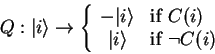
Grover's algorithm can then be used to solve the equation ![]() while
besides the fact that a solution exists and that it is unique,
no additional knowledge about
while
besides the fact that a solution exists and that it is unique,
no additional knowledge about ![]() is required.
is required.
Usually, the implementation of
![]() will be complicated
enough as not to allow an efficient algebraic solution, but
since the inner structure of
will be complicated
enough as not to allow an efficient algebraic solution, but
since the inner structure of ![]() doesn't matter for the
algorithm, we can easily implement a test query with the
solution
doesn't matter for the
algorithm, we can easily implement a test query with the
solution ![]() as
as
qufunct query(qureg x,quvoid f,int n) {
  int i;

  for i=0 to #x-1 {     // x -> NOT (x XOR n)
    if not bit(n,i) { Not(x[i]); }
  }
  CNot(f,x);            // flip f if x=1111..
  for i=0 to #x-1 {     // x <- NOT (x XOR n)
    if not bit(n,i) { !Not(x[i]); }
  }
}
|
A more realistic application would be the search for an encryption
key in a known-plaintext attack.
With ![]() being the known plaintext to the ciphertext
being the known plaintext to the ciphertext ![]() , a
QCL implementation could look like this:
, a
QCL implementation could look like this:
qufunct encrypt(int p,quconst key,quvoid c) { ... }

qufunct query(int c,int p,quconst key,quvoid f) {
  int i;
  quscratch s[blocklength];

  encrypt(p,key,s);
  for i=0 to #s-1 {     // s -> NOT (s XOR p)
    if not bit(p,i) { Not(x[i]); }
  }
  CNot(f,x);            // flip f if s=1111..
}
|
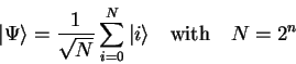
The solution space of a ![]() bit query condition
bit query condition ![]() is
is ![]() .
On a quantum computer, this search space can be implemented as
a superposition of all eigenstates of an
.
On a quantum computer, this search space can be implemented as
a superposition of all eigenstates of an ![]() qubit register, i.e.
qubit register, i.e.
 |
(4.2) |
 |
(4.3) |
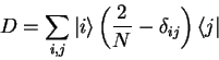
The main loop of the algorithm consists of two steps
 |
(4.4) |
 |
(4.5) |
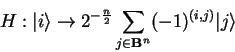
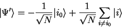
Since only one eigenvector
![]() is supposed to match the search
condition
is supposed to match the search
condition ![]() , the conditional phase shift will turn the
initial even superposition into
, the conditional phase shift will turn the
initial even superposition into
 |
(4.6) |
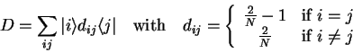
The effect of the diffusion operator on an arbitrary eigenvector
![]() is
is
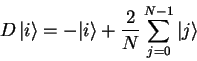 |
(4.7) |
 |
(4.8) |
| (4.9) |
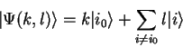
If the above loop operator ![]() is repeatedly applied to
the initial superposition
is repeatedly applied to
the initial superposition
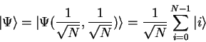 |
(4.10) |
 |
(4.11) | ||
 |
(4.12) |
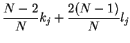
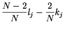
Using the substitution
![]() the solution
of the above system can be written in closed form.
the solution
of the above system can be written in closed form.
| (4.13) | |||
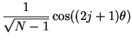 |
(4.14) |
The probability ![]() to measure
to measure ![]() is given as
is given as ![]() and
has a maximum at
and
has a maximum at
![]() .
Since for large lists,
.
Since for large lists,
![]() we can assume
that
we can assume
that
![]() and
and
![]() and the number of iterations
and the number of iterations ![]() for a maximum
for a maximum
![]() is about
is about
![]() with
with
![]() (due to rounding errors).
Alternatively, if we are content with
(due to rounding errors).
Alternatively, if we are content with ![]() , then
, then
![]() iterations will do.
iterations will do.
If we choose to formulate the query as quantum function with
a flag qubit ![]() to
allow for a strictly classical implementation, as
suggested in 4.1.1, then the operator
to
allow for a strictly classical implementation, as
suggested in 4.1.1, then the operator ![]() can
be constructed as
can
be constructed as
| (4.15) |
Using the Hadamard Transform ![]() (see 3.4.4.3) and a
conditional phase rotation
(see 3.4.4.3) and a
conditional phase rotation
![]() ,
the diffusion operator
,
the diffusion operator
 |
(4.16) |
 |
(4.17) |
 |
(4.18) |
Using the ![]() operator from 3.4.7.4 and
a conditional phase gate
operator from 3.4.7.4 and
a conditional phase gate ![]() we can implement the
diffusion operator as
we can implement the
diffusion operator as
operator diffuse(qureg q) {
  Mix(q);               // Hadamard Transform
  Not(q);               // Invert q
  CPhase(pi,q);         // Rotate if q=1111..
  !Not(q);              // undo inversion
  !Mix(q);              // undo Hadamard Transform
}
|
In fact, the above operator implements ![]() , but since overall
phases make no physical difference, this doesn't matter.
, but since overall
phases make no physical difference, this doesn't matter.
By using the above, we can now give a QCL implementation of the complete algorithm:
procedure grover(int n) {
  int l=floor(log(n,2))+1;        // no. of qubits
  int m=ceil(pi/8*sqrt(2^l));     // no. of iterations
  int x;
  int i;
  qureg q[l];
  qureg f[1];

  {
    reset;
    Mix(q);             // prepare superposition
    for i= 1 to m {     // main loop
      query(q,f,n);     // calculate C(q)
      CPhase(pi,f);     // negate |n>
      !query(q,f,n);    // undo C(q)
      diffuse(q);       // diffusion operator
    }
    measure q,x;        // measurement
    print "measured",x;
  } until x==n;
}
|
qcl> grover(500); : 9 qubits, using 9 iterations : measured 500 qcl> grover(123); : 7 qubits, using 5 iterations : measured 74 : measured 123 qcl> grover(1234); : 11 qubits, using 18 iterations : measured 1234 |